
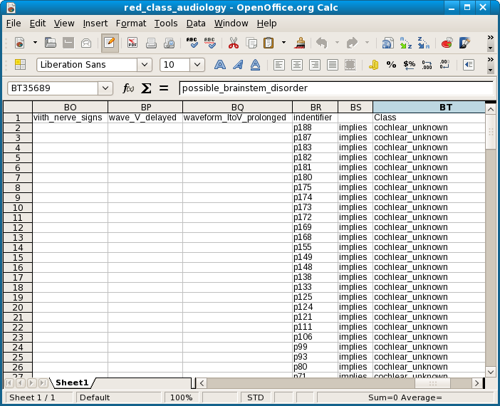
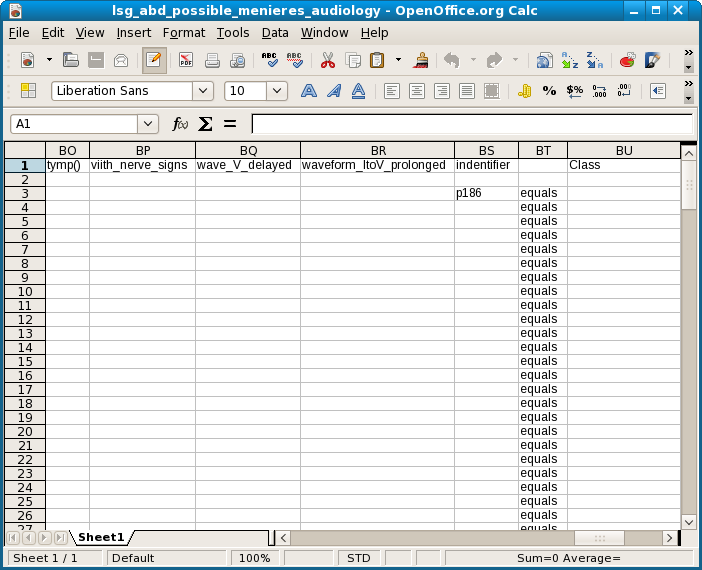
The next data set was originally donated to the UCI Machine learning repository by Professor Jergen at Baylor College of Medicine and later adapted somewhat (see the relevant section at the UCI site). The version used here contains only 200 rows but 71 columns. Of those 71 one is called Class, which has 24 values, presumably the diagnoses. Unlike the mushroom data table, there is also a column called indentifier which identifies each individual patient. (My typographical error here and with another header was discovered rather late and therefore not corrected.) Because of my unfamiliarity with the subject and the medical terminology, no attempt was made at interpretation or clarification of these data. Here is a screen shot of the OO Calc spreadsheet.

The .csv file was imported into a SQLite database to facilitate testing. The reduction with Class as consequent attribute took 32 minutes, which is about 1.5 minute for each of the 24 values. There are no ambiguous rules for Class. The number of reductions is no less than 37231! This is a screenshot.
As expected, because each patient identifier uniquely determines a diagnosis, all identifiers turn up in the reduction as singleton predictors.
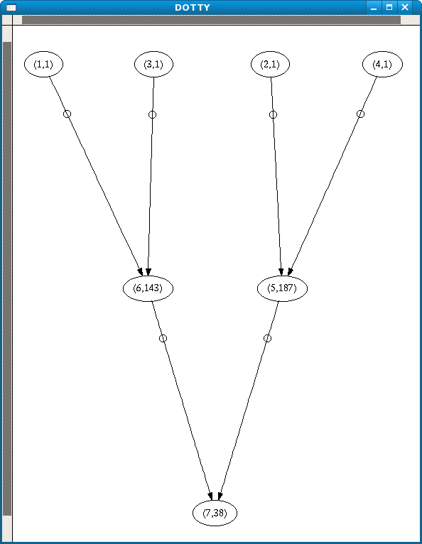
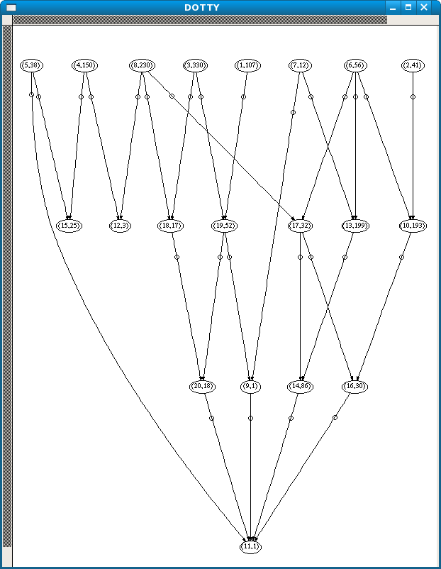
Subsequent abductions took negligible time. This is the screenshot of the graph for the value possible_brainstem_disorder. The first number is the node, and the second is the number of equivalence classes in that node.
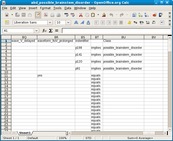
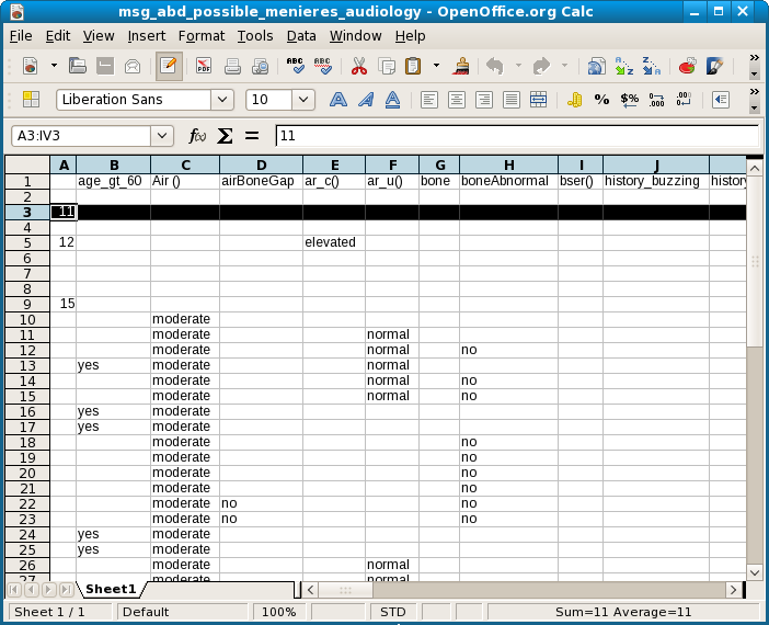
This is the corresponding abduction spreadsheet. The node numbers (not shown here) are in the leftmost column. The predicate conjunctions for each representative of the equivalence group denoted by the node are in the rows.
As expected, each patient identifier turns up as a least general rule for possible_brainstem_disorder. According to the graph nodes 1 and 3, which correspond to patients p198 and p120, each imply node 6, which consists of 143 equivalences. This in its turn implies node 7, with 38 equals. Nodes 2 and 4 (p141 and p91) imply node 5 with 187 equivalence groups, but this also implies node 7.
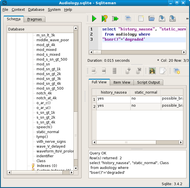
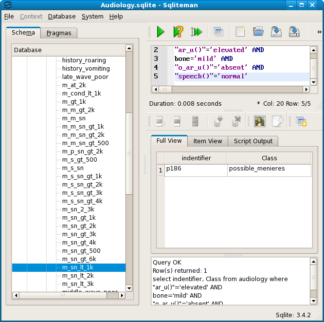
The shortest description of node 6 is a singleton, bser() = degraded. So first we test p198 and p120. This is the screenshot for p198.
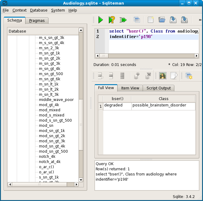
p120 returns the same result, but p141 and p91 do not. For those the class is still possible_brainstem_disorder but bser() is ? (a question mark).
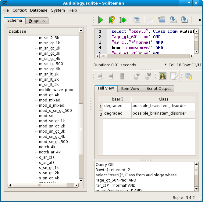
Next we check that the result, bser() = degraded, indeed implies one of the 38 equivalent descriptions of node 7. The shortest description is history_nausea = yes and static_normal = no.
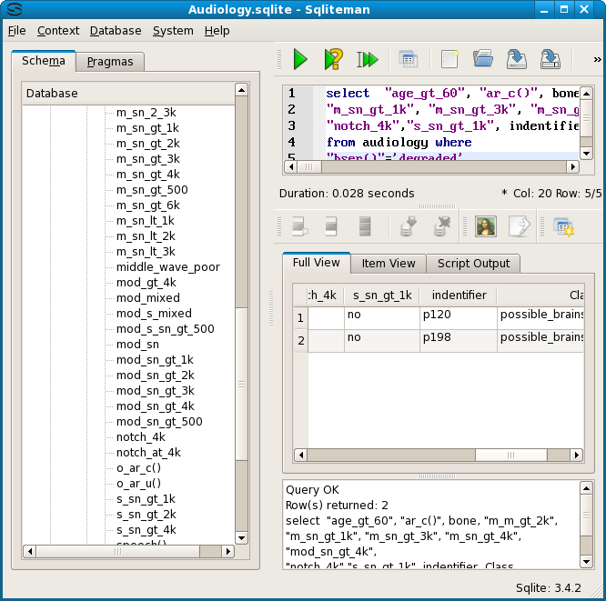
Additionally we test the equivalence of the shortest description of node 6 with the longest description of node 6, which consists of 10 attribute values. For emphasis the indentifier column has been added to the display selection.
We also test the reverse. These two descriptions do indeed denote the same rows from the source table.
The dependencies for nodes 2 and 4 (p141 and p91) were also tested. Both imply node 5, which also has a singleton as its shortest reperentative, waveform_ItoV_prolonged= yes. Both tests passed, as did the subsequent test for the most general node 7.
So, to summarize, Emping found that two patients show bser() = degraded, and two others show waveform_ItoV_prolonged = yes, but both these disjunct symptoms show history_nausea = yes and static_normal = no. Furthermore, because the data table includes a unique patient identifier, each patient could be traced. Furthermore, we can test that bser() and waveform_ItoV_prolonged are indeed disjunct. An SQL query showed that waveform_ItoV = yes implies bser() = ? (a question mark), while bser() = degraded implies waveform_ItoV = no. The diagnosis for all 4 cases is possible_brainstem_disorder.
The next screenshot shows the graph for Class = possible_menieres.
As in the case for possible_brainstem_disorder, the individual patients show up as the least general equivalences, at the top of the graph. Here is a screenshot of the least general in the spreadsheet.
Unlike the cases for possible_brainstem_disorder, where the 4 patients all showed up on a single line, these identifiers are all equivalent to many different conjunctions of symptems. Node 1, p186, is just one of 107. Testing the second of these descriptions indeed showed an equivalence.
For possible_menieres there are 3 most general equivalence classes, nodes 11, 12 and 15.
Interestingly, as can be seen from the graph, node 11 covers all other nodes except one, node 4. Looking at the spreadsheet for the abduction, we see that this is the equivalence group of p98.
Node 11 is not only represented by just one description, this is also a singleton, history_fluctuating = yes. In the database we indeed find 7 rows for this attribute value, all possible_menieres, and all identifiers except p98. We also found a history_fluctuating = no for this single case, as well as possible_menieres, of course.
Next we test the trace in the graph, starting with node 1. We take the shortest available representative for each case.
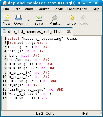
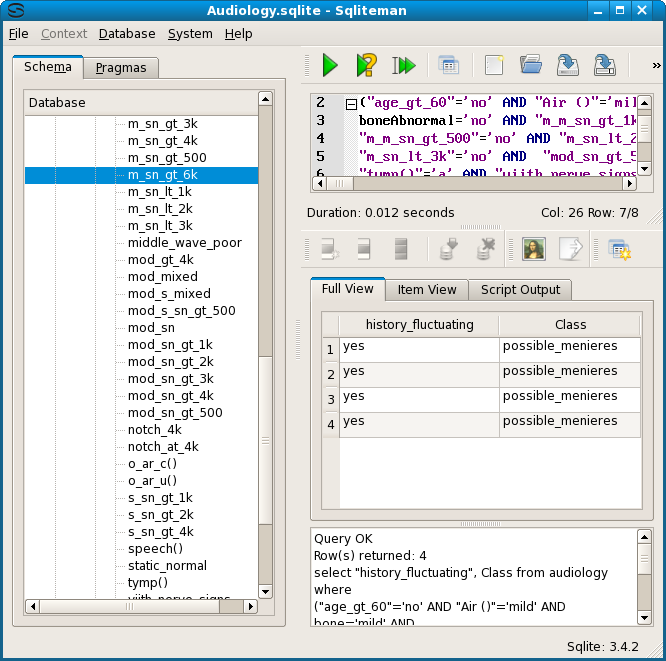
First, node 1 goes to node 19. This test passed. Now node 19 goes to node 20 or node 9. Node 9 is just one line, with singleton property m_sn_lt_1k = yes. So the 6 attribute-values of node 19, taken together, should imply this result. This test passed, with 2 rows. The same query should also imply node 20, which has 12 attribute-values as its shortest representation. This also passed, with 2 rows in the result. Now both of these nodes go to node 11. So, we have to test the 12 attribute values of node 20 for history_fluctuating = yes, and the 1 attribute value of node 9 for the same result. Both passed, each with 3 rows. Here is the query with an OR of both.
This is a screenshot of the result
The differing row numbers highlight an important aspect of the equivalence classes of reduced rules. They are not necessarily disjunct, even though the graph intuitively suggest this. In the case of the audiology table, where each row has a unique (patient) identifier, the least general rules will always be disjunct, because a patient can (supposedly) have only one diagnosis. So, for the audiology graphs, the number of rows in each node can be found by counting the least general ones which point to it. However, this does not have to be the case for all nominal data tables.
Many other abduction graphs for the audiology Class values do not show the structure we have found for these two cases. We have demonstrated, however, that if such a structure exists Emping can be used to find and to analyze relations between patients, symptoms and diagnosis.

